Machine learning (ML) is at the core of our strategy to accelerate drug discovery for novel cancer treatments, and scalable ML inference is at the core of our ability to rapidly analyze large molecular datasets. To scale up ML inference in a cost- and time-effective way, we built a parallel inference system using the Ray framework and AWS Spot instances. Ray offered us an easy way to develop highly parallel Python applications, and AWS Spot instances offered maximum scale at minimum cost. This blog post focuses on how we leveraged Python’s asyncio library to send and manage many parallel inference requests while analyzing large datasets.

Note: This blog post is a case study of asyncio at Reverie rather than a general introduction to the library. For further information about the library, a great blog post building asyncio from the ground up can be found here: https://tenthousandmeters.com/blog/python-behind-the-scenes-12-how-asyncawait-works-in-python/

System Constraints and Design

Before jumping into the code, we’ll first outline some of the constraints for the system that led to our design:

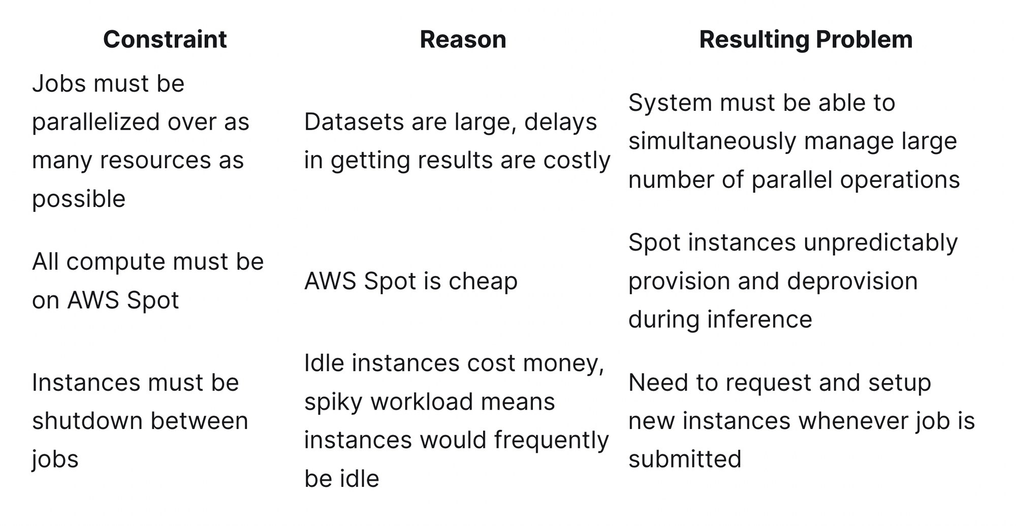
These constraints led to two primary design goals:

1. Support for massive number of parallel operations
2. Quick adaption to Spot instance availability

Parallel Operations

Our parallel operations are farmed out to our Ray cluster, so they can be thought of as “very long I/O” operations that require minimal local compute. To simultaneously manage the large number of parallel operations during inference, we considered three standard Python options: multi-core (multiprocessing), multi-thread (threading), and coroutines (asyncio).

1. multiprocessing: In theory, it offered the greatest potential for parallelism in Python because we could leverage more than one CPU core and escape the GIL. In practice, subprocess overhead was considerable, and it capped the number of operations we could manage at a relatively low number.
2. threading: Much lighter weight than subprocesses, but the number of threads in a single process (and therefore the number of parallel operations) was still capped at a relatively low number.
3. asyncio: Very, very lightweight with support for orders of magnitude more concurrent operations than multi-threading. This was the clear choice for managing our non-CPU bound Ray operations. Other advantages were Ray’s native integration with asyncio and syntactic simplicity vs. threading or multiprocessing.

Spot Instance Availability

While the concurrency framework choice was easy, we still needed to ensure the system responded to changes in available resources. As an example of how responsiveness affected performance, a request for ten AWS Spot instances might provision in two batches, half after one minute and half after three minutes. To avoid wasting time or money, we wanted to start sending molecules for inference as soon as the first set of instances provisioned. However, to maximize parallelism and shorten the job, we also wanted to expand inference to the second set of instances as soon as they provisioned. The diagram below shows the performance improvement of supporting this staggered provisioning behavior.

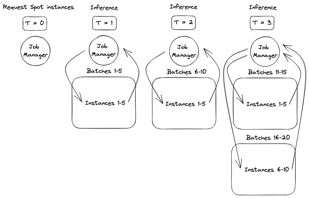
The next portion of the blog post will introduce the basic inference system components, demonstrate a basic parallelization strategy that is not responsive to this type of staggered provisioning, and then show a more advanced system with asyncio that responds effectively to these changes. Finally, simulation results will be presented demonstrating the performance and cost advantages of responding to dynamic worker availability.

Sample Python Pseudocode for a Basic Parallel System

A sample inference system worker along with the procedure to deploy and run inference through it is shown below. Details of the Ray API are beyond the scope of this blog post (Ray docs can be found here), but as a summary, the first .remote() call gives us a handle to a deployed ModelWorker instance on the Ray cluster, and the second .remote() sends an RPC to the remote ModelWorker instance to run inference. The result of that RPC call is waited on and obtained by ray.get().

# Basic system components
import ray

# Inference worker
@ray.remote
class ModelWorker:
    def __init__(self):
        # download and load model...
        pass

    def predict(self, molecule):
        # model magic happens...
        return predictions

    # used later to know when the worker has fully deployed
    def heartbeat(self):
        return

# Deploying the worker
worker = ModelWorker.remote()

# Running inference on the worker
results = ray.get(worker.predict.remote(molecule))

Using those components, we made a basic parallel system by deploying many workers at once and sending one input batch to each worker.

# Approach #1: Basic parallelism
molecules = list(range(10))

# Deploy one worker for each input batch
# This line does not block, .remote() calls return immediately
worker_futures = [ModelWorker.remote() for _ in range(len(molecules))]

# Send each input batch to a worker, wait for all batches to complete
# This line does not block, but each `predict` RPC will not execute until
# its underlying `worker` object is ready.
prediction_futures = [worker.predict.remote(molecule) for worker, molecule in zip(worker_futures, molecules)]

# Block until all predictions are complete
results = ray.get(prediction_futures)

While this approach was parallel and therefore much faster than running using one worker, there were still a few problems:

1. Job Length: Job was only as fast as its slowest request. Even if 99/100 workers deployed instantly and completed, if worker #100 required a new Spot instance to spin up, the entire job had to wait for that worker to complete.
2. Resource Waste: Idle workers didn’t terminate until the job was complete, preventing the instances they ran on from spinning down. Idle workers also couldn’t be reused to process molecules that were still in the inference queue.

Sample Python Pseudocode for Improved System with Asyncio

With a new strategy made easy with asyncio utilities, we resolved these issues. The strategy was as follows:

1. Manage a pool of available workers instead of creating a worker for each molecule.
2. Send molecules to workers as they become available (e.g., after successfully deploying or finishing an earlier task).
3. If a worker dies, reassign the molecule it was working on to another worker in the pool and start a replacement worker deploying in the background.
4. Scale down the pool as time passes to ensure pool size is never greater than the amount of remaining input batches.

With the worker pool strategy, we could ensure that regardless of what size the pool grew or shrunk to, we could always ensure it was fully utilized, minimizing cost and maximizing speed. The snippet below shows one way to implement this strategy with asyncio (note that for brevity, fault tolerance/retry functionality and pool scale down are not shown):

# Approach #2: Worker pool strategy (runnable by adding basic system component code)
available_workers = asyncio.Queue()
input_idx_to_result = {}
input_molecules = list(range(10))
all_tasks = set()

async def deploy_worker():
    worker = ModelWorker.remote()
    await worker.heartbeat.remote()  # block until worker is actually deployed
    await available_workers.put(worker)

async def run_inference(input_idx, molecule):
    # Get worker, run inference, return worker to pool
    worker = await available_workers.get()

    results = await worker.predict.remote(molecule)
    input_idx_to_result[input_idx] = results

    await available_workers.put(worker)

# Deploy workers and send prediction requests
# NOTE: This for loop is entirely non-blocking and completes very quickly
for idx, molecule in enumerate(input_molecules):
    deploy_task = asyncio.create_task(deploy_worker())
    deploy_task.set_name(f"deploy-{idx}")
    all_tasks.add(deploy_task)

    inference_task = asyncio.create_task(
        run_inference(input_idx=idx, molecule=molecule)
    )
    inference_task.set_name(f"inference-{idx}")
    all_tasks.add(inference_task)

# All of the deploy and inference tasks are now in flight! 
# As soon as workers become available, they can be used.
# Deployed workers can also be reused if others are slow to deploy.
# Contrast this to Approach #1, which couldn't reuse deployed workers.

pending = all_tasks
while not len(input_idx_to_result) == len(input_molecules):
    done, pending = await asyncio.wait(pending)

    for completed_task in done:
        try:
            completed_task.exception()
        except:
            task_name = completed_task.get_name()
            # handle error and retry inference/re-deploy worker...

Performance Improvement Simulation

To give a sense of how performance improves, the simulation below compares using an inference system allowing worker reuse (like Approach #2) to a system that uses a 1:1 input:worker mapping (like Approach #1). Specifically, it examines the improvement in Approach #2’s job length and cost in response to the following parameters:

1. Number of input molecules to the job
2. Maximum time to provision a new worker node

To provide a more fair comparison point for the simulation, Approach #1 was improved by placing all the __init__ and predict logic into one function, then deploying that function as a stateless Ray Task instead of a stateful Ray Actor. Because Ray Tasks release their resources on completion for other Ray Tasks to use, they avoid the idle worker problem and allow nodes to be reused. However, because Ray Tasks are stateless, each one must download and load the model to run inference on its assigned input. This adds overhead equal to (# inputs) * (time and cost to download and load model) over the course of the job, assuming one input per task.

Some additional assumptions in the simulation are:

1. Idle/unneeded workers can be spun down before the full job is complete (to lower cost).
2. A job requests, at start time, resources sufficient to spin up 1 worker for each input (to maximize parallelism).
   1. Note that the job may not get all its requested resources before the job completes, depending on how long the resources take to provision.
3. Both modes can reuse nodes that have spun up, but only the simulation modeling Approach #2 can re-use model workers.
   1. This is because Approach #2 still uses stateful Ray Actors that hold the model in memory after loading it once, rather than stateless Ray Tasks that destroy their resources on completion.
4. Inference takes 1 Time Unit (TU).
5. Creating a model worker on a deployed node takes 1 TU.
6. Running a node for 1 TU takes 1 Cost Unit (CU).
7. Each node has capacity for 1 worker.
8. Each node takes 3 TU to setup after provisioning (e.g., for container downloading).

Simulation results are shown below.

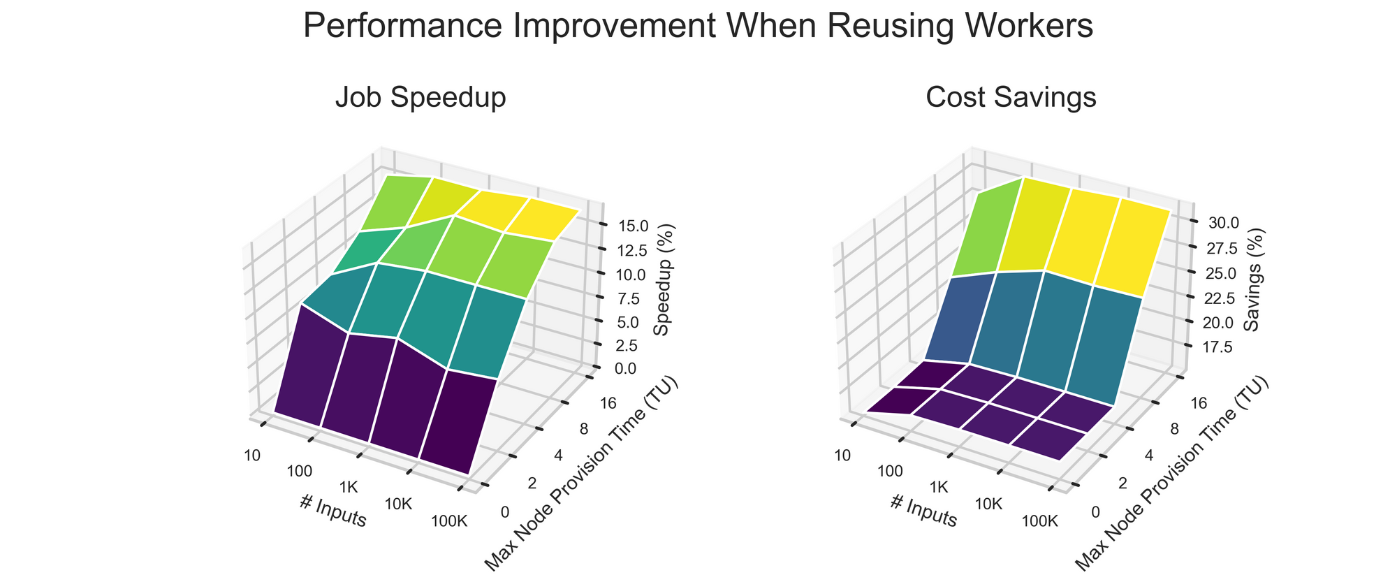
The takeaways from the simulation are as follows:

1. Number of Input Batches Minimally Impacts Improvement.
   1. Time: The outsize impact of a single slow node spinup becomes smaller and smaller as the number of workers increases.
   2. Cost: Reusing an existing worker is cheaper than creating a new one (no node or worker setup overhead), but as more and more workers are used, the fraction of batches sent to old workers levels off.
2. Longer Node Start Times Increase Worker Reuse Advantage.
   1. Time: Reusing workers enables progress during time steps the other system spends deploying or waiting for resources.
   2. Cost: As max node start time goes to infinity, Approach #2 begins to resemble the case of using a single worker for the entire job. Using a single worker amortizes node/worker setup time across all batches and thus is cost-optimal from a dollar perspective, but it’s extremely slow and thus negatively impacts users’ research speed.

Conclusion

Here, we worked through a few iterations of a parallel inference system, settling on one that uses asyncio to manage many concurrent prediction operations and maximize worker utilization. A simulation of the two closest matched systems demonstrated the time and cost advantages of a flexible “worker pool” system, and we’ve seen internally the advantages it provides for granular error handling and iterative pool scale-down. Overall, asyncio provided us an easy way to manage our scaled up inference workloads while keeping run time and cost growth to a minimum.

We are Hiring!

If this type of work excites you, check out our careers page! Our team includes a mix of industry-experienced engineering and biotech professionals. We're actively hiring engineers across our tech stack, including Machine Learning Engineers, Senior Data Scientists, and Full Stack Engineers to work on exciting challenges critical to our approach to developing life-saving cancer drugs. You will work with a YC-backed team that is growing in size and scope. You can read more about us at reverielabs.com, and please reach out if you're interested in learning more.